KNN and SVM

K Nearest Neighbours

KNN is predicting the unknown value of the point based on the values nearby.

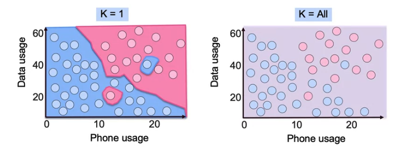
Decision Boundary

KNN does not provide a correct K such that the right value of K depends on which error metric is most importnat. Elbow method is a cmmon way to find the right value of K. We chose K from the kink of the error curve. It is choosing majority vote.

KNN Regression is prediction based on mean value of K neighbors. But slow computation because many distance calculation and does not generate insight innto data generating process.

Distant Measurement

• Euclidean distance L2
• Manhattan Distance L1

Scale for Distance Measurement

When the scale of X is small relative to the scale of Y, clustering the data may be inaccurate. Curse of dimensionality

from sklearn.neighbors import KNeighborsClassifier
knn = KNeighborsClassifier(n_neighbors=3) #by default, euclidean distance, also related to scale
knn = knn.fit(X_train, y_train)
y_pred = knn.predict(X_test) #fit(x,y) and fit_transform(single value)

from sklearn.neighbors import KNeighborsRegressor

Support Vector Machines

Cost function for SVM is the cost of misclassification (Lost class).

SVM is Linear model

SVM or Support Vector Machine is a linear model for classification and regression problems. It can solve linear and non-linear problems and work well for many practical problems. The idea of SVM is simple: The algorithm creates a line or a hyperplane which separates the data into classes.
$e.g.) z = X^2 +Y^2$ transfroms non-linear data into linearly-separable data.
Thus we can classify data by adding an extra dimension to it so that it becomes linearly separable and then projecting the decision boundary back to original dimensions using mathematical transformation. But finding the correct transformation for any given dataset isn’t that easy. Thankfully, we can use kernels in sklearn’s SVM implementation to do this job.

Regularixation

Outlier Sensitivity
Out of two outliers disturbs the model. For example, a point close to the other group that is not belonging to makes SVM to draw the line close to the other group. So in this case, misclassification should be admitted
So, we use regularization below.

$$J(\beta_i) = SVMCost(\beta_i) + \frac{1}{C}\sum_i \beta_i$$

Smaller C, the more regularized.

from sklearn.svm import LinearSVC, SVC(?) # LinearSVM for regression.
LinSVC = LinearSVC(C=1.0, class_weight=None, dual=True, fit_intercept=True,
                    penalty='l2', random_state=None)
LinSVC = LinSVC.fit(X_train, y_train)
y_pred = LinSVC.predict(X_test)

Kernels

Kernels map hyperplane to the higher dimensional space. Utilizes similarity metrics (e.g. Gaussian Kernel, Radial Basis Function) to find out which point is closest to the new point. I.E. apply Kernel for all data points.
Higher C and gamma means less regulazation and more complex models

from sklearn.svm import SVC
svc = SVC(kernel='rbf', C=1.0, gamma=0.1)
svc = svc.fit(X_train, y_train)
y_pred = svc.predict(X_test)

Faster Kernel Transformation

Nystroem. n_components is the number of samples and use cross-validation for hyperparameters

from sklearn.kernel_approximation import Nystroem
Nystroem = Nystroem(kernel='rbf', gamma=1.0, n_components=100)
X_kernel = Nystroem.fit_transform(X_train)
X_test = Nystroem.transform(X_test)

from sklearn.kernel_approximation import RBFSampler
RBFSampler = RBFSampler(gamma=1, n_components=100)
X_kernel = RBFSampler.fit_transform(X_train)
X_test = RBFSampler.transform(X_test)

Machine Learning Workflow

Features	Data	Model Choice
many(~10K)	Small(~1K rows)	Simplle, Logistic, LinearSVC
few(<100)	Medium(<10K rows)	SVC with RBF
few(<100)	Large(>100K rows)	ADd features, Logistic, LinarSVC or Kernel Approx