Decision Tree

Decision Tree

Building a decision tree

1. select a feature
2. split the data into two groups.
3. Split until
   1. the leaf node are pure (only one class remains)
   2. The maximum depth of the tree is reached
   3. A performance metric is achieved

The decision tree uses a greedy search to find the best split at each step. The Best Split is the split that minimizes the information.\

Splitting Criteria

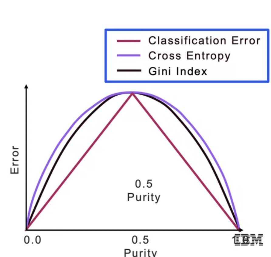
Classification Error Equation

$$E(t) = 1-max_i[P(i|t)]$$

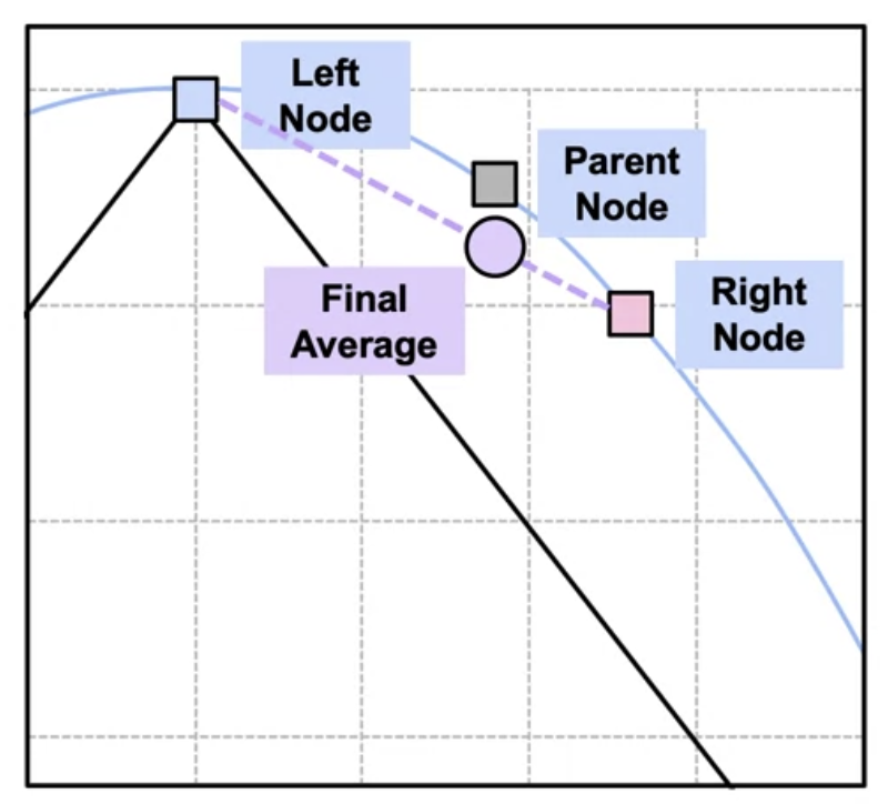
But this metric does not change overall Error rate when parent node error is compared with weighted average of child node error.\

Thus, we use Entroy Equation

$$H(t) = -\sum_i[P(i|t)log_2(P(i|t))]$$

The Gini index is also used

$$G(T) = 1-\sum_i P(i|t)^2$$

Characteristics of a Decision Tree

Since DT easily ovefitted, we use pruning. Prune based on classification error threshold. Pros is that it is easy to interpret and implement.

from sklearn.tree import DecisionTreeClassifier
DTC = DecisionTreeClassifier(criterion='Gini', max_Features=10, max_depth=3)
DTC.fit(X_train, y_train)
y_pred = DTC.predict(X_test)

Ensemble

Combining prediction to reduce variance. We can reduce variance by pruning but pruning may lost generlization

Bagging

Bagging is bootstrap aggregating.Bagging is a tree ensemble that combines the prediction of several trees that were trained on bootstrap samples of the data. The underlying idea is that a model that averages the predictions of multiple models reduces the variance of a single model and has high chances to generalize well when scoring new data.
Pasting is when bootstrapping is held without replacement.

Heterogeneous input data allowed, no preprocessing needed

Out-of-Bag Score

OOB Scoring is the chance of not being selected
When there are $n$ samples, the chance for a sample not being selected is $1 - \frac{1}{n}$. Thus, probability of a sample being not selected after n draws is $(1-\frac{1}{n})^n$. When $n \to \infty$, the probability converges to $1/e = 0.3678$.

from sklearn.ensemble import BaggingClassifier
bc = BaggingClassifier(base_estimator=DTC, n_estimators=10, max_samples=0.5, max_features=0.5)
bc.fit(X_train, y_train)

Random Forest

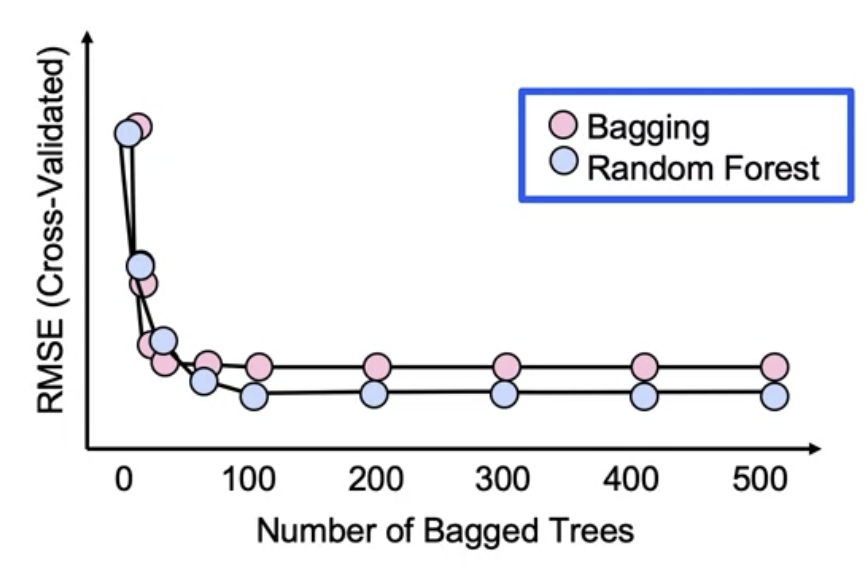
The bagged variance is $\sigma^2 /n$. However bootstrap samples are correlated $\rho \sigma^2 + \frac{1-\rho}{n} \sigma^2$.
We introduce more randomness???? to solve this. Use random subset of features ofr each tree, so that classification $\sqrt{m}$ amd regression $m/3$.

from sklearn.ensemble import BaggingClassifier

from sklearn.ensemble import RandomForestClassifier
rf = RandomForestClassifier(n_estimators=10, max_features=0.5, max_depth=3)
rf.fit(X_train, y_train)
y_pred = rf.predict(X_test)

from sklearn.ensamble import ExtraTreesClassifier
ec = ExtraTreesClassifier(n_estimators=10, max_features=0.5, max_depth=3)
ec.fit(X_train, y_train)
y_pred = ec.predict(X_test)

Boosting

Weighting different trees differently to imporve. So we lower the weights of the records that the first model got right, and increase the weights of the ones that are wrongly classified and that’s the major idea here in boosting. And we put $\lambda$ to control the weight of each trees. Using a learning rate $< 1.0$ helps lessening the overfitting cases.
Boosting fit entire data set and base trees created successively, using residuals from previous models. Also this up-weight miscalssified points.

Gradient Boosting Functions

1. 0-1 loss function ignores observations that were correctly classified. The shape of this loss function makes it difficult to optimize.
2. Adaboost is an adaptive boosting using $e^{-marginal}$ as the loss function. 3. Gradient boosting uses $log(1+e^{-margin})$ as the loss function.

Hyperparameters

• learning rate for shrinkage
• Stochastic gradient boosting subsample to use fraction of data for base learners
• max_features number of features to use for each base learner But since we cannot parallel trees, needs logn time.

from sklearn.ensemble import AdaBoostClassifier
from sklearn.ensemble import GradientBoostingClassifier
gbc = GradientBoostingClassifier(learning_rate = 0.1,
        n_estimators=10, max_features=0.5, max_depth=3)
abc = AdaBoostClassifier(base_estimator=gbc, n_estimators=10, learning_rate=0.1)
# we set max_dept from gbc.
gbc.fit(X_train, y_train)
y_pred = gbc.predict(X_test)

Stacking

Stacking is a way to combine multiple models, but should be aware of increasing model complexity. The model prediction can be done by voting or with another model.

Hard voting vs Soft voting

from sklearn.ensamble import VotingClassifier
vc = VotingClassifier(estimators=[('rf', rf), ('gbc', gbc), ('abc', abc)], voting='hard')
vc.fit(X_train, y_train)
y_pred = vc.predict(X_test)

from sklearn.emsable import StakingClassifier #work similarly