Machine Learning on Apple stock daily return

import numpy as np
import pandas as pd
import os
import matplotlib.pyplot as plt
%matplotlib inline
import seaborn as sns

1. Data

aapl = pd.read_csv('./data/aapl.csv')
X = aapl.drop(['Date','daily_ret'], axis=1)
y = aapl['daily_ret']

aapl.columns

Index(['Date', 'Close', 'Volume', 'Lo', 'HO', 'CO', 'support_low',
       'support_open', 'support_high', 'std20', 'std120', 'std_open20',
       'std_high20', 'std_intra', 'ma20', 'ma120', 'daily_ret', 'd_mom',
       '3d_mom', '5d_mom', '20d_mom', '252d_mom', 'AAPL_factor2',
       'AAPL_factor1', 'change_wti', 'Lo_wti', 'HO_wti', 'CO_wti',
       'change_nasdaq', 'Lo_nasdaq', 'HO_nasdaq', 'CO_nasdaq',
       'Close_bond_10y', 'high6m_bond_10y', 'Close_bond_2y', 'high6m_bond_2y',
       'change_itw', 'Lo_itw', 'HO_itw', 'CO_itw', 'Close_bond_1m',
       'high6m_bond_1m', 'Close_bond_1y', 'high6m_bond_1y', 'Close_vix',
       'change_vix', 'Lo_vix', 'HO_vix', 'CO_vix', 'high6m_vix', 'high1y_vix',
       'Close_sp500', 'change_sp500', 'Lo_sp500', 'HO_sp500', 'CO_sp500',
       'high6m_sp500', 'high1y_sp500', 'y', 'm', 'd', 'vix_cat',
       'vix_change_cat', 'sp500_cat', 'sp500_change_cat'],
      dtype='object')

1-1 Determining Normality

BoxCox Transformation

## from scipy.stats.mstats import normaltest ## D'Agostino K^2 Test
## from scipy.stats import boxcox ## Not doing this since it's time series data and not normally distributed

## ## Adding boxcox value
## aapl_cut = aapl.drop(['Date','daily_ret'], axis=1)
## nomres = normaltest(aapl_cut)
## aapl_cut = aapl_cut.iloc[:,np.where(nomres[0] > 0.05)[0].tolist()]
## for i in aapl_cut.columns:
##     bc_res = boxcox(aapl_cut[i])
##     aapl['box_'+i] = bc_res[0]

Using dummy variables

Making dummy variable based on categorized data

• vix, vix change
• sp500, sp500 change

opt = True
if opt:
    one_hot_encode_cols = aapl.dtypes[aapl.dtypes == aapl.vix_cat.dtype]  ## filtering by string categoricals
    one_hot_encode_cols = one_hot_encode_cols.index.tolist()  ## list of categorical fields

    ## Do the one hot encoding
    df = pd.get_dummies(aapl, columns=one_hot_encode_cols, drop_first=True).reset_index(drop=True)

    ## ## Combination of dummy variables: Not useful since it takes a lot of computing power
    ## pd.options.mode.chained_assignment = None
    ## temp = pd.DataFrame()
    ## for i in [one_hot_encode_cols[0],one_hot_encode_cols[2]]:
    ##     lists = df.columns[1:]
    ##     for name in lists:
    ##         if name in "daily_ret":
    ##             continue
    ##         if name[:-2] not in one_hot_encode_cols:
    ##             for j in range(2,5):
    ##                 temp[name+'*'+i+'_'+str(j)] = df[name]*df[i+'_'+str(j)]
    ## df = pd.concat([df, temp], axis=1)
else:
    df = aapl
    
def singular_test(data):
    dc = data.corr()
    non = (dc ==1).sum() !=1
    return dc[non].T[non]

singular_test(df)

2. Sklearn learing model

from sklearn.preprocessing import StandardScaler, PolynomialFeatures
from sklearn.metrics import r2_score, confusion_matrix, classification_report, \
    accuracy_score, precision_score, recall_score, f1_score
from sklearn.model_selection import TimeSeriesSplit, cross_validate, \
    RandomizedSearchCV, GridSearchCV, train_test_split
from sklearn.pipeline import Pipeline

Testing learning model

def evaluate(model, X, y, cv, 
             scoring = ['r2', 'neg_mean_squared_error'],
             validate = True):
    if validate:
        verbose = 0
    else:
        verbose = 2
    scoring = ['r2', 'neg_mean_squared_error']
    cv_results = cross_validate(model, X, y, cv=cv,
        scoring = scoring, verbose=verbose)
    return cv_results

def regress_test(data, regressor, params = None,
            target ='daily_ret', window = 120, pred_window = 30):
    ## training with 6month(120days) and predict 3month(60days)
    X = data.drop([target], axis=1)
    y = data[target]
    tscv = TimeSeriesSplit() ## n_splits=_num_batch

    pf = PolynomialFeatures(degree=1)
    alphas = np.geomspace(50, 800, 20)
    scores=[]
    for alpha in alphas:
        ridge = Ridge(alpha=alpha, max_iter=100000)

        estimator = Pipeline([
            ('scaler', StandardScaler()),
            ("polynomial_features", pf),
            ("ridge_regression", ridge)])

        r2, mse = evaluate(estimator, X, y, cv = tscv)
        scores.append(np.mean(r2))
    plt.plot(alphas, scores)

## regress_test(df, Ridge())

Learning Model

What is the problem here?

from tqdm import tqdm

def Xy(df, target, cls):
    if cls:
        return df.drop([target, 'Date'], axis=1), df[target] >0
    else:
        return df.drop([target, 'Date'], axis=1), df[target]

def execute_CV(model, param_grid, X, y, cv, poly = None, gridsearch = True, **kwargs):
    if poly != None:
        # when both polynomial features and parameter grid are used
        scores = {}
        poly_able = (X.dtypes != 'uint8').values
        X_poly, X_non = X.iloc[:, poly_able], X.iloc[:, ~poly_able]
        for i in tqdm(poly):
            X2 = PolynomialFeatures(degree=i).fit_transform(X_poly)
            X2 = np.concatenate([X2, X_non], axis=1)
            if gridsearch:
                CV_ = GridSearchCV(model, param_grid, cv=cv, verbose =1, **kwargs)
            else:
                CV_ = RandomizedSearchCV(model, param_grid, cv=cv, verbose =1, **kwargs)
            CV_.fit(X2, y)
            scores[CV_.best_score_] = (i, CV_)
            
        mxx = scores[max(scores.keys())]
        print(mxx[0])
        return mxx[1]
    
    else:
        ## When only parameter grid are used
        if gridsearch:
            CV_ =  GridSearchCV(model, param_grid, cv=cv, verbose = 1, **kwargs)
        else:
            CV_ = RandomizedSearchCV(model, param_grid, cv=cv, verbose =1, **kwargs)
        CV_.fit(X,y)
        print('Best score:', CV_.best_score_)
        return CV_

def class_report(y_true, y_pred):
    print('Accuracy:', accuracy_score(y_true, y_pred))
    print('F1:', f1_score(y_true, y_pred))
    return classification_report(y_true, y_pred, output_dict=True)
    


def measure_error(y_train, y_test, pred_train, pred_test, label):
    train =  pd.Series({'accuracy':accuracy_score(y_train, pred_train),
                      'precision': precision_score(y_train, pred_train),
                      'recall': recall_score(y_train, pred_train),
                      'f1': f1_score(y_train, pred_train)},
                      name='train')
    
    test = pd.Series({'accuracy':accuracy_score(y_test, pred_test),
                    'precision': precision_score(y_test, pred_test),
                    'recall': recall_score(y_test, pred_test),
                    'f1': f1_score(y_test, pred_test)},
                    name='test')

    return pd.concat([train, test], axis=1)


from colorsetup import colors, palette
import seaborn as sns
sns.set_palette(palette)
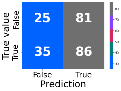
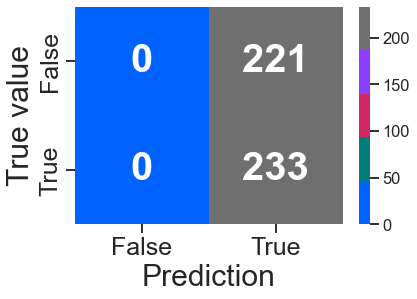
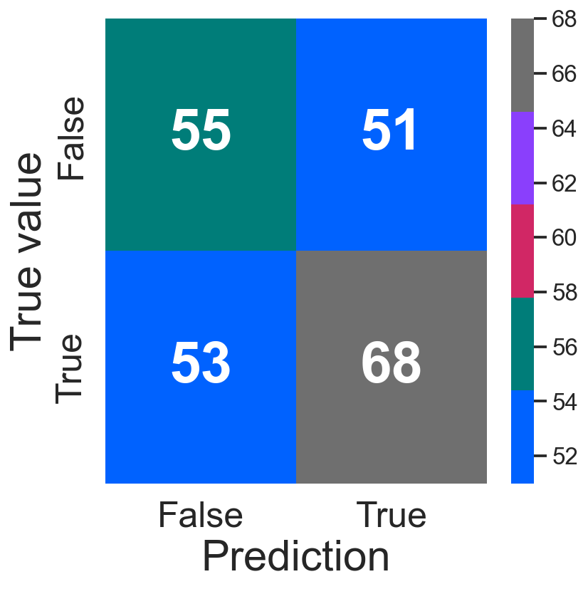
def confusion_plot(y_true, y_pred):
    sns.set_palette(sns.color_palette(colors))
    _, ax = plt.subplots(figsize=None)
    ax = sns.heatmap(confusion_matrix(y_true, y_pred), 
                     annot=True, fmt='d', cmap=colors, 
                     annot_kws={"size": 40, "weight": "bold"})
    labels = ['False', 'True']
    ax.set_xticklabels(labels, fontsize=25);
    ax.set_yticklabels(labels, fontsize=25);
    ax.set_ylabel('True value', fontsize=30);
    ax.set_xlabel('Prediction', fontsize=30)
    return ax

def learning(data: pd.DataFrame, regressor, params = None, clss = False, pred = False,
            n_jobs = None, poly = None, scores = None, Date = 'Date', gridsearch = True,
            target ='daily_ret', window = 400, pred_window = 15, prnt = True, refit = True):

    ## training with 6month(120days) and predict 3month(60days)
    if pred == True:
        data, data_pred = train_test_split(data, test_size=0.1, shuffle = False)
    X, y = Xy(data, target, clss)

    tscv = TimeSeriesSplit() #n_splits=int(data.shape[0]), max_train_size=window
    
    if params != None:
        cvres =  execute_CV(regressor, params, X, y, tscv, poly = poly, gridsearch = gridsearch,
                                scoring= scores, n_jobs = n_jobs, refit = refit)
        if pred:
            X_pred, y_pred = Xy(data_pred, target, clss)
            if prnt:
                if clss != True:
                    print(r2_score(y_pred, cvres.predict(X_pred)))
                print(confusion_plot(y_pred>0, cvres.predict(X_pred)>0))
            rpt = class_report(y_pred, cvres.predict(X_pred))
            return cvres, rpt
        else:
            return cvres, None
    else:
        ## cross validation only with polynomial features
        if poly != None:
            scores = {}
            poly_able = (X.dtypes != 'uint8').values
            X_poly, X_non = X.iloc[:, poly_able], X.iloc[:, ~poly_able]
            for i in tqdm(poly):
                X2 = PolynomialFeatures(degree=i).fit_transform(X_poly)
                X2 = np.concatenate([X2, X_non], axis=1)
                cv_results = cross_validate(regressor, X2, y, cv = tscv,
                                            verbose=1)
                scores[i] = cv_results
                if prnt:
                    print(scores)
            return regressor.fit(X2, y), scores
        else:
            ## no cross validation
            res = []
            reg = regressor.fit(X, y)
            if pred:
                X_pred, y_pred = Xy(data_pred, target, clss)
                if prnt:
                    if clss != True:
                        res.append(r2_score(y_pred, reg.predict(X_pred)))
                        print(confusion_plot(y_pred>0, reg.predict(X_pred)>0))
                    else:
                        res.append(class_report(y_pred, reg.predict(X_pred)))
                    print(confusion_plot(y_pred>0, reg.predict(X_pred)>0))
            else:
                res = evaluate(reg, X, y, tscv, clss)
            return reg, res

3. Regression

from sklearn.linear_model import LinearRegression, Lasso, Ridge, \
    ElasticNet
from sklearn.ensemble import GradientBoostingRegressor

Ridge Regression

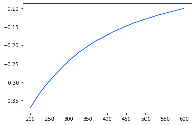
lr = Ridge(max_iter=3000)
params = {
    'ridge_regression__alpha': np.geomspace(200, 600, 10)
}
regressor = Pipeline([
    ("ridge_regression", lr)])

reg = learning(data = df, regressor = regressor, params = params, pred = True)
res = reg.cv_results_

Fitting 5 folds for each of 10 candidates, totalling 50 fits
Best score: -0.004782872997843679
0.0018543351779481965
AxesSubplot(0.125,0.125;0.62x0.755)

print(plt.plot(res['param_ridge_regression__alpha'], res['mean_test_score']))

[<matplotlib.lines.Line2D object at 0x157a00eb0>]

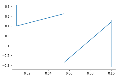
lr = Lasso(max_iter=3000)
params = {
    'ridge_regression__alpha': np.geomspace(10, 400, 10)
}
regressor = Pipeline([
    ("ridge_regression", lr)])

reg = learning(data = df, regressor = regressor, params = params, pred= True)
res = reg.cv_results_
plt.plot(res['param_ridge_regression__alpha'], res['mean_test_score'])

Fitting 5 folds for each of 10 candidates, totalling 50 fits
Best score: -0.0015480943621106746
-0.0002423279793632993
AxesSubplot(0.125,0.125;0.62x0.755)





[<matplotlib.lines.Line2D at 0x28795ba00>]

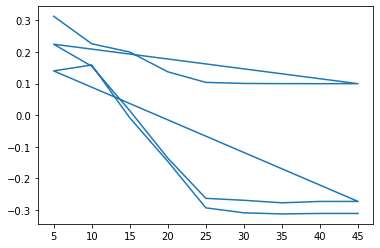
lr = ElasticNet(max_iter=50000)
params = {
    'ElasticNet__alpha': np.geomspace(10, 150, 10),
    'ElasticNet__l1_ratio': np.linspace(0.1, 0.3, 10)
}
regressor = Pipeline([
    ("ElasticNet", lr)])

reg = learning(data = df, regressor = regressor, params = params, pred=  True)
res = reg.cv_results_
## print(plt.plot(res['param_ElasticNet__alpha'], res['mean_test_score']))
print(plt.plot(res['param_ElasticNet__l1_ratio'], res['mean_test_score']))

Fitting 5 folds for each of 100 candidates, totalling 500 fits
Best score: -0.0015480943621106746
-0.0002423279793632993
AxesSubplot(0.125,0.125;0.62x0.755)
[<matplotlib.lines.Line2D object at 0x28633eca0>]

Latex stuff

lr = LinearRegression()
reg = learning(data = df, regressor = lr)
print(pd.DataFrame(reg).to_latex())

\begin{tabular}{lrrrr}
\toprule
{} &  fit\_time &  score\_time &    test\_r2 &  test\_neg\_mean\_squared\_error \\
\midrule
0 &  0.005983 &    0.006344 & -25.157695 &                    -0.007231 \\
1 &  0.083999 &    0.002470 &  -1.262275 &                    -0.000328 \\
2 &  0.016528 &    0.002174 &   0.339044 &                    -0.000204 \\
3 &  0.014251 &    0.007031 &  -1.576393 &                    -0.001622 \\
4 &  0.016815 &    0.003716 &   0.262219 &                    -0.000214 \\
\bottomrule
\end{tabular}



/var/folders/1t/_7p_zm4x449blqs7bvqvb0rm0000gn/T/ipykernel_66451/1592972210.py:3: FutureWarning: In future versions `DataFrame.to_latex` is expected to utilise the base implementation of `Styler.to_latex` for formatting and rendering. The arguments signature may therefore change. It is recommended instead to use `DataFrame.style.to_latex` which also contains additional functionality.
  print(pd.DataFrame(reg).to_latex())

df.shape

(2266, 57)

lr = LinearRegression()
regressor = Pipeline([
    ("standard_scaler", StandardScaler()),
    ('poly', PolynomialFeatures(degree=2)),
    ("ridge_regression", lr)])
reg = learning(data = df, regressor = regressor)
print(pd.DataFrame(reg).to_latex())

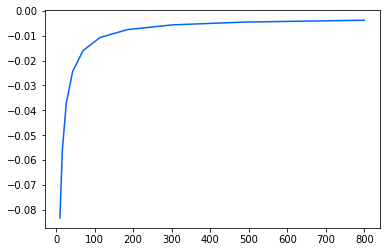
lr = Ridge(max_iter=3000)
params = {
    'ridge_regression__alpha': np.geomspace(10, 800, 10)
}
regressor = Pipeline([
    ("ridge_regression", lr)])

reg = learning(data = df, regressor = regressor, params = params,
               scores = ['r2', 'neg_mean_squared_error'], refit = 'r2')
res = reg.cv_results_
print(reg.best_params_)
print(plt.plot(res['param_ridge_regression__alpha'].data, res['mean_test_r2']))

Fitting 5 folds for each of 10 candidates, totalling 50 fits
Best score: -0.0037675812365856264
{'ridge_regression__alpha': 800.0}
[<matplotlib.lines.Line2D object at 0x2878eea90>]

SGD Regression

• Requires alpha, rmse, l1 ratio from elasticnet?

GBR

lr = GradientBoostingRegressor(random_state=717)
params = {
    'GBR__learning_rate': np.linspace(0.01, 0.1, 3),
    'GBR__max_depth': np.arange(5, 50, 5),
}
regressor = Pipeline([
    ("GBR", lr)])

reg = learning(data = df, regressor = regressor, params = params)
res = reg.cv_results_
print(reg.best_params_)
plt.plot(res['param_GBR__learning_rate'], res['mean_test_score'])

Fitting 5 folds for each of 27 candidates, totalling 135 fits
0.312927684076205
{'GBR__learning_rate': 0.01, 'GBR__max_depth': 5}





[<matplotlib.lines.Line2D at 0x298c75160>]

plt.plot(res['param_GBR__max_depth'], res['mean_test_score'])

[<matplotlib.lines.Line2D at 0x298686700>]

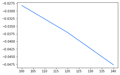
lr = GradientBoostingRegressor(random_state=717, 
                               learning_rate = 0.005, max_depth = 5)
params = {
    ## 'GBR__max_depth': np.arange(2, 10, 2),
    'GBR__n_estimators': np.arange(100, 150, 20),
}
regressor = Pipeline([
    ("GBR", lr)])

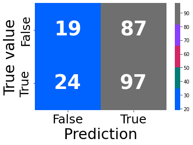
reg = learning(data = df, regressor = regressor, params = params, pred = True)
res = reg.cv_results_
print(reg.best_params_)

Fitting 5 folds for each of 3 candidates, totalling 15 fits
Best score: -0.028233698083682923
-0.017464138185920186
AxesSubplot(0.125,0.125;0.62x0.755)
{'GBR__n_estimators': 100}

plt.plot(res['param_GBR__n_estimators'], res['mean_test_score'])

[<matplotlib.lines.Line2D at 0x169d50d60>]

3. Classification

from sklearn.metrics import confusion_matrix, accuracy_score, classification_report, f1_score
from sklearn.linear_model import LogisticRegression
from sklearn.neighbors import KNeighborsClassifier
from sklearn.tree import DecisionTreeClassifier
from sklearn.ensemble import GradientBoostingClassifier, RandomForestClassifier

3-1 Basic classification models

3-1-1 Logistic Regression

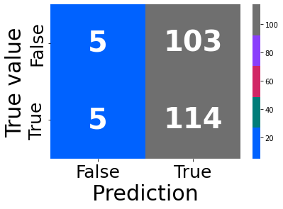
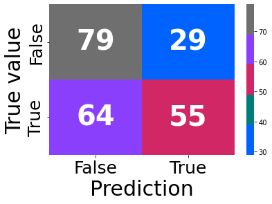
lr = LogisticRegression(solver='liblinear', max_iter= 3000, penalty = 'l1')
params = {
    'log__C': np.linspace(10, 40, 5),
}
regressor = Pipeline([
    ("log", lr)])

reg, rpt = learning(data = df, regressor = regressor, params = params, \
    clss = True, pred = True)
res = reg.cv_results_
print(reg.best_params_)
plt.plot(res['param_log__C'], res['mean_test_score'])

Fitting 5 folds for each of 5 candidates, totalling 25 fits
Best score: 0.5893805309734513
Accuracy: 0.6387665198237885
F1: 0.6796875
AxesSubplot(0.125,0.125;0.62x0.755)
{'log__C': 32.5}





[<matplotlib.lines.Line2D at 0x2866f62e0>]

reg

              precision    recall  f1-score   support

       False       0.56      0.81      0.66       108
        True       0.71      0.41      0.52       119

    accuracy                           0.60       227
   macro avg       0.63      0.61      0.59       227
weighted avg       0.64      0.60      0.59       227

3-1-2 Tree based modelm

from io import StringIO
from IPython.display import Image
from sklearn.tree import export_graphviz
import pydotplus

## Estimate dtc model and report outcomes
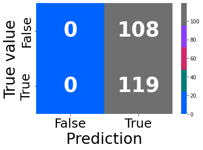
dt1 = DecisionTreeClassifier()
dt1, rpt = learning(data = df, regressor = dt1,
    clss = True, pred = True, prnt = False)

## Estimate dtc model and report outcomes
dtc = DecisionTreeClassifier()
params = {'max_depth':range(1, dt1.tree_.max_depth+1, 2),
              'max_features': range(1, len(dt1.feature_importances_)+1)}

reg, rpt = learning(data = df, regressor = dtc, params = params,\
    clss = True, pred = True)
print(reg.best_params_)

Fitting 5 folds for each of 639 candidates, totalling 3195 fits
Best score: 0.6466076696165193
AxesSubplot(0.125,0.125;0.62x0.755)
Accuracy: 0.6167400881057269
F1: 0.5538461538461539
{'max_depth': 3, 'max_features': 25}

reg.best_par

res = reg.cv_results_
plt.plot(res['param_max_depth'].data, res['mean_test_score'])

[<matplotlib.lines.Line2D at 0x176a475b0>]

#### BEGIN SOLUTION
## Create an output destination for the file
dot_data = StringIO()

export_graphviz(reg.best_estimator_, out_file=dot_data, filled=True)
graph = pydotplus.graph_from_dot_data(dot_data.getvalue())

## View the tree image
filename = 'wine_tree_prune.png'
graph.write_png(filename)
Image(filename=filename) 
#### END SOLUTION

3-1-3 KNN

## Estimate KNN model and report outcomes
knn = KNeighborsClassifier()
params = {
    'knn__n_neighbors': np.arange(50, 150, 5),
    'knn__weights': ['uniform', 'distance'],
}

model = Pipeline([
    ("knn", knn)])

reg = learning(data = df, regressor = model, params = params,\
    clss = True, pred = True)
res = reg.cv_results_
print(reg.best_params_)

Fitting 5 folds for each of 40 candidates, totalling 200 fits
Best score: 0.5386430678466076
              precision    recall  f1-score   support

       False       0.42      0.24      0.30       106
        True       0.51      0.71      0.60       121

    accuracy                           0.49       227
   macro avg       0.47      0.47      0.45       227
weighted avg       0.47      0.49      0.46       227

Accuracy: 0.4889867841409692
F1: 0.5972222222222222
AxesSubplot(0.125,0.125;0.62x0.755)
{'knn__n_neighbors': 145, 'knn__weights': 'uniform'}

train, test = train_test_split(df, test_size=0.2, shuffle = False)
X_train = train.drop(['daily_ret', 'Date'], axis=1)
y_train = train['daily_ret']>0
X_test = test.drop(['daily_ret','Date'], axis=1)
y_test = test['daily_ret']>0


max_k = 40
f1_scores = list()
error_rates = list() ## 1-accuracy

for k in range(1, max_k):
    
    knn = KNeighborsClassifier(n_neighbors=k, weights='distance')
    knn = knn.fit(X_train, y_train)
    
    y_pred = knn.predict(X_test)
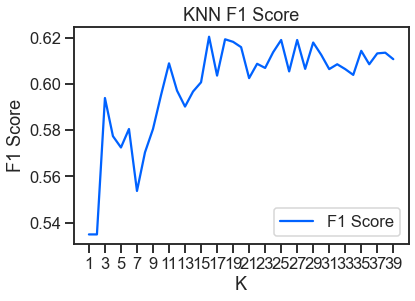
    f1 = f1_score(y_pred, y_test)
    f1_scores.append((k, round(f1_score(y_test, y_pred), 4)))
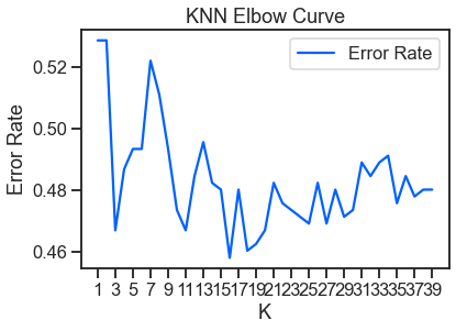
    error = 1-round(accuracy_score(y_test, y_pred), 4)
    error_rates.append((k, error))
    
f1_results = pd.DataFrame(f1_scores, columns=['K', 'F1 Score'])
error_results = pd.DataFrame(error_rates, columns=['K', 'Error Rate'])

## Plot F1 results
sns.set_context('talk')
sns.set_style('ticks')

plt.figure(dpi=300)
ax = f1_results.set_index('K').plot(color=colors[0])
ax.set(xlabel='K', ylabel='F1 Score')
ax.set_xticks(range(1, max_k, 2));
plt.title('KNN F1 Score')
## plt.savefig('knn_f1.png')

Text(0.5, 1.0, 'KNN F1 Score')




<Figure size 1800x1200 with 0 Axes>

## Plot Accuracy (Error Rate) results
sns.set_context('talk')
sns.set_style('ticks')

plt.figure(dpi=300)
ax = error_results.set_index('K').plot(color=colors[0])
ax.set(xlabel='K', ylabel='Error Rate')
ax.set_xticks(range(1, max_k, 2))
plt.title('KNN Elbow Curve')

Text(0.5, 1.0, 'KNN Elbow Curve')




<Figure size 1800x1200 with 0 Axes>

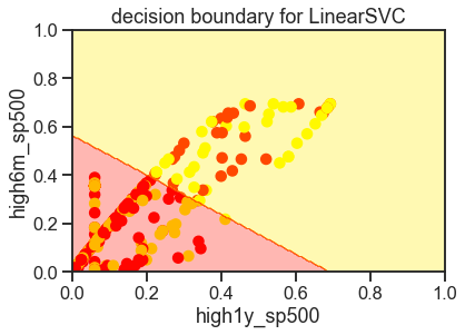
3-2 Linear Decision boundary

from sklearn.svm import LinearSVC

X = df.drop(['daily_ret', 'Date'], axis=1)
y = df['daily_ret']>0

fields = list(X.columns[:-1]) 
correlations = abs(X[fields].corrwith(y))
correlations.sort_values(inplace=True)
fields = correlations.map(abs).sort_values().iloc[-2:].index
X_sub = X[fields]

LSVC = LinearSVC()
LSVC.fit(X_sub.values, y)

X_color = X_sub.sample(300, random_state=45)
y_color = y.loc[X_color.index]
y_color = y_color.map(lambda r: 'red' if r == 1 else 'yellow')
ax = plt.axes()
ax.scatter(
    X_color.iloc[:, 0], X_color.iloc[:, 1],
    color=y_color, alpha=1)
## -----------
x_axis, y_axis = np.arange(0, 1.005, .005), np.arange(0, 1.005, .005)
xx, yy = np.meshgrid(x_axis, y_axis)
xx_ravel = xx.ravel()
yy_ravel = yy.ravel()
X_grid = pd.DataFrame([xx_ravel, yy_ravel]).T
y_grid_predictions = LSVC.predict(X_grid)
y_grid_predictions = y_grid_predictions.reshape(xx.shape)
ax.contourf(xx, yy, y_grid_predictions, cmap=plt.cm.autumn_r, alpha=.3)
## -----------
ax.set(
    xlabel=fields[0],
    ylabel=fields[1],
    xlim=[0, 1],
    ylim=[0, 1],
    title='decision boundary for LinearSVC');

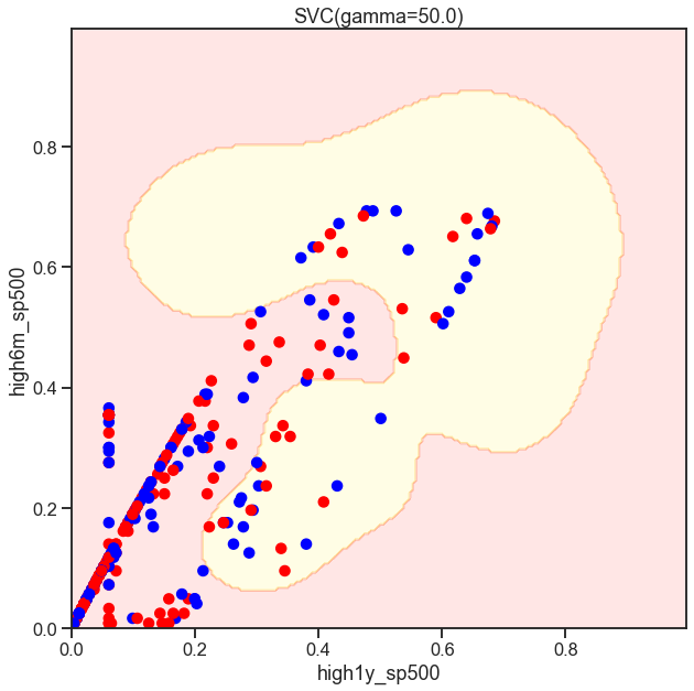
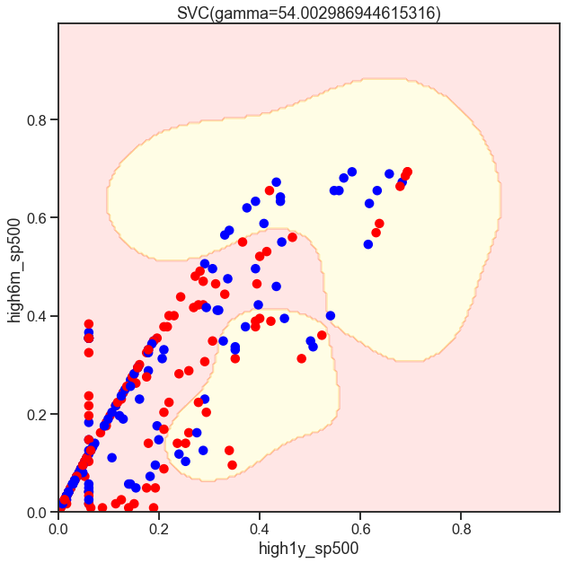
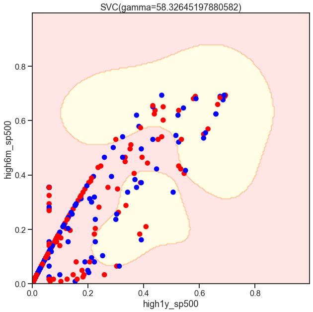
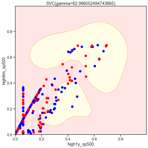
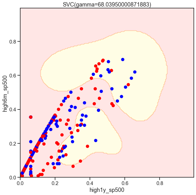
def plot_decision_boundary(estimator, X, y):
    estimator.fit(X.values, y)
    X_color = X.sample(300)
    y_color = y.loc[X_color.index]
    y_color = y_color.map(lambda r: 'red' if r == 1 else 'blue')
    x_axis, y_axis = np.arange(0, 1, .005), np.arange(0, 1, .005)
    xx, yy = np.meshgrid(x_axis, y_axis)
    xx_ravel = xx.ravel()
    yy_ravel = yy.ravel()
    X_grid = pd.DataFrame([xx_ravel, yy_ravel]).T
    y_grid_predictions = estimator.predict(X_grid.values)
    y_grid_predictions = y_grid_predictions.reshape(xx.shape)

    fig, ax = plt.subplots(figsize=(10, 10))
    ax.contourf(xx, yy, y_grid_predictions, cmap=plt.cm.autumn_r, alpha=.1)
    ax.scatter(X_color.iloc[:, 0], X_color.iloc[:, 1], color=y_color, alpha=1)
    ax.set(
        xlabel=fields[0],
        ylabel=fields[1],
        title=str(estimator))

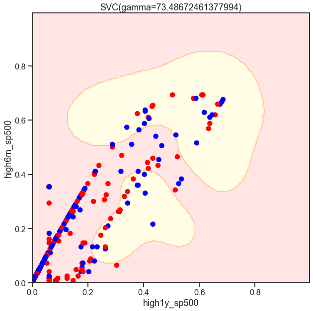
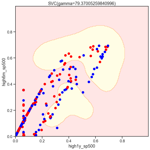
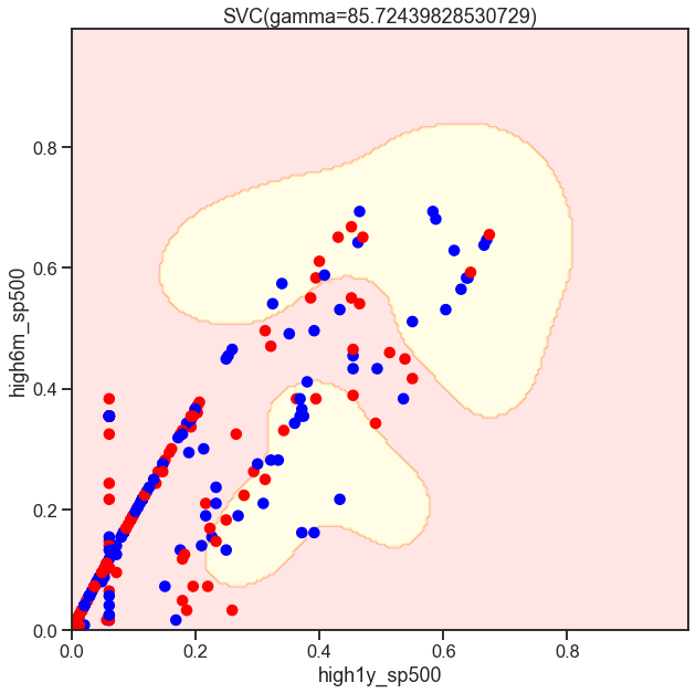
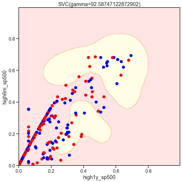
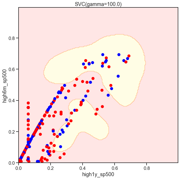
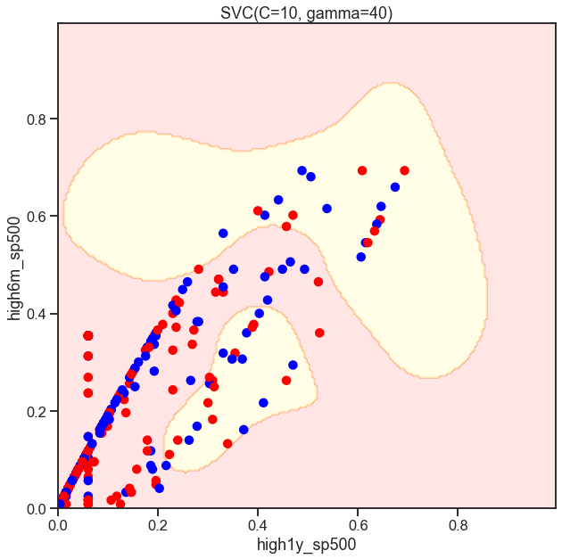
from sklearn.svm import SVC

gammas = np.geomspace(50, 100, num=10)
for gamma in gammas:
    SVC_Gaussian = SVC(kernel='rbf', gamma=gamma)
    plot_decision_boundary(SVC_Gaussian, X_sub, y)

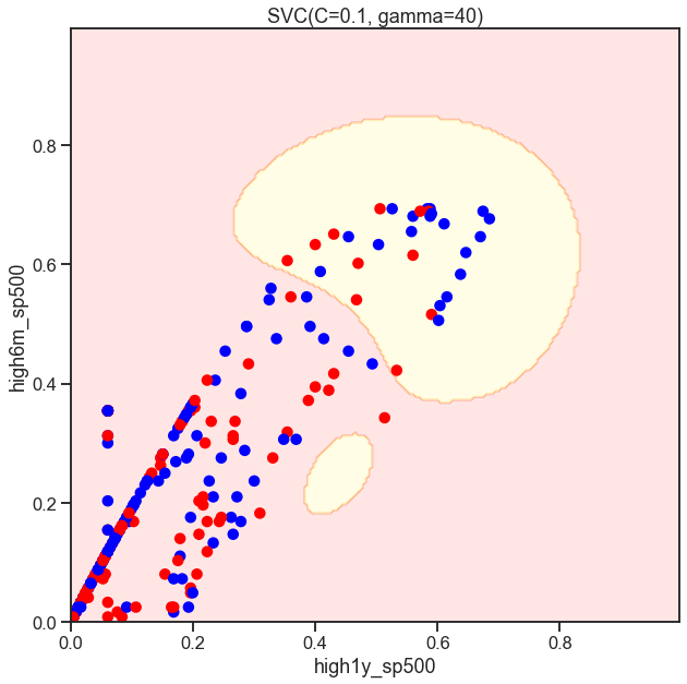
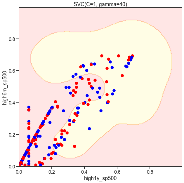
Cs = [.1, 1, 10]
for C in Cs:
    SVC_Gaussian = SVC(kernel='rbf', gamma=40, C=C)
    plot_decision_boundary(SVC_Gaussian, X, y)

/Users/hun/miniforge3/envs/hun/lib/python3.9/site-packages/sklearn/base.py:450: UserWarning: X does not have valid feature names, but SVC was fitted with feature names
  warnings.warn(
/Users/hun/miniforge3/envs/hun/lib/python3.9/site-packages/sklearn/base.py:450: UserWarning: X does not have valid feature names, but SVC was fitted with feature names
  warnings.warn(
/Users/hun/miniforge3/envs/hun/lib/python3.9/site-packages/sklearn/base.py:450: UserWarning: X does not have valid feature names, but SVC was fitted with feature names
  warnings.warn(

Classifcation

• SVC, nystroem converge time
• Tree model

from sklearn.kernel_approximation import Nystroem
from sklearn.svm import SVC
from sklearn.linear_model import SGDClassifier

X = df.drop(['daily_ret', 'Date'], axis=1)

kwargs = {'kernel': 'rbf'}
svc = SVC(**kwargs)
nystroem = Nystroem(**kwargs)
sgd = SGDClassifier()

%%timeit
svc.fit(X, y)

158 ms ± 894 µs per loop (mean ± std. dev. of 7 runs, 10 loops each)

%%timeit
X_transformed = nystroem.fit_transform(X)
sgd.fit(X_transformed, y)

50.2 ms ± 15.8 ms per loop (mean ± std. dev. of 7 runs, 10 loops each)

%%timeit
X2_transformed = nystroem.fit_transform(X2)
sgd.fit(X2_transformed, y2)

train_test_full_error
#### END SOLUTION

	train	test
accuracy	1.0	0.513216
precision	1.0	0.522388
recall	1.0	0.600858
f1	1.0	0.558882

from sklearn.model_selection import GridSearchCV

param_grid = {'max_depth':range(1, dt.tree_.max_depth+1, 2),
              'max_features': range(1, len(dt.feature_importances_)+1)}

GR = GridSearchCV(DecisionTreeClassifier(random_state=42),
                  param_grid=param_grid,
                  scoring='recall',
                  n_jobs=-1)

GR = GR.fit(X_train, y_train)

GR.best_estimator_.tree_.node_count, GR.best_estimator_.tree_.max_depth

(3, 1)

y_train_pred_gr = GR.predict(X_train)
y_test_pred_gr = GR.predict(X_test)

train_test_gr_error = pd.concat([measure_error(y_train, y_train_pred_gr, 'train'),
                                 measure_error(y_test, y_test_pred_gr, 'test')],
                                axis=1)
train_test_gr_error

	train	test
accuracy	0.529801	0.513216
precision	0.529801	0.513216
recall	1.000000	1.000000
f1	0.692641	0.678311

confusion_plot(y_test, y_test_pred_gr)

<AxesSubplot:xlabel='Prediction', ylabel='True value'>

3-3 Classification Ensamble

## Estimate dtc model and report outcomes
gbc = GradientBoostingClassifier(random_state=777, n_iter_no_change= 10)
gbc, rpt = learning(data = df, regressor = gbc, clss = True, pred = True, prnt = False)

gbc2 = GradientBoostingClassifier(random_state=777, n_iter_no_change = 10, n_estimators= gbc.n_estimators_+10)
params = {'max_depth':range(3, len(gbc.feature_importances_), 2),
          'max_features': range(1, gbc.max_features_+1)}
reg, rpt = learning(data = df, regressor = gbc2, params = params, clss = True, pred = True)

res = reg.cv_results_
print(reg.best_params_)

Fitting 5 folds for each of 2414 candidates, totalling 12070 fits
Best score: 0.6525073746312684
AxesSubplot(0.125,0.125;0.62x0.755)
Accuracy: 0.5903083700440529
F1: 0.541871921182266
{'max_depth': 3, 'max_features': 45}

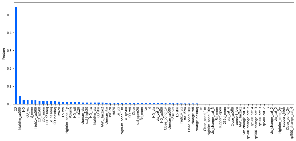
model = reg.best_estimator_
feature_imp = pd.Series(model.feature_importances_, index=df.drop(['Date','daily_ret'],axis=1).columns).sort_values(ascending=False)

ax = feature_imp.plot(kind='bar', figsize=(16, 6))
ax.set(ylabel='Relative Importance');
ax.set(ylabel='Feature');

4. Unsupervised

aapl2 = pd.read_csv('./data/aapl2.csv').dropna()
## float_columns = [i for i in aapl2.columns if i not in ['Date']]
## no_cols = [i for i in aapl.columns if i not in float_columns]
## aapl2 = pd.merge(aapl[no_cols], aapl2, on='Date', how = 'left')
float_columns = [i for i in aapl2.columns if aapl2.dtypes[i] != object]

## sets backend to render higher res images
%config InlineBackend.figure_formats = ['retina']
import numpy as np, pandas as pd, seaborn as sns, matplotlib.pyplot as plt
from sklearn.preprocessing import scale, StandardScaler, MinMaxScaler
from sklearn.cluster import KMeans, AgglomerativeClustering

4-1 K-means clustering

plt.rcParams['figure.figsize'] = [6,6]
sns.set_style("whitegrid")
sns.set_context("talk")

## helper function that allows us to display data in 2 dimensions an highlights the clusters
## def display_cluster(X,kmeans):
##     plt.scatter(X[:,0], 
##                 X[:,1])

##     ## Plot the clusters 
##     plt.scatter(kmeans.cluster_centers_[:, 0], 
##                 kmeans.cluster_centers_[:, 1], 
##                 s=200,                             ## Set centroid size
##                 c='red')                           ## Set centroid color
##     plt.show()
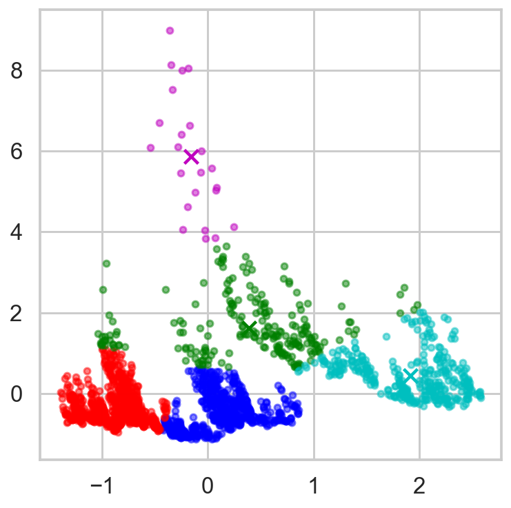
def display_cluster(X,km=[],num_clusters=0):
    color = 'brgcmyk'
    alpha = 0.5
    s = 20
    if num_clusters == 0:
        plt.scatter(X[:,0],X[:,1],c = color[0],alpha = alpha,s = s)
    else:
        for i in range(num_clusters):
            plt.scatter(X[km.labels_==i,0],X[km.labels_==i,1],c = color[i],alpha = alpha,s=s)
            plt.scatter(km.cluster_centers_[i][0],km.cluster_centers_[i][1],c = color[i], marker = 'x', s = 100)

X_cdf = aapl2[['Close_sp500', 'Close_vix']]
cdf = StandardScaler().fit(X_cdf).transform(X_cdf)

num_clusters = 5
km = KMeans(n_clusters=num_clusters, n_init=10) ## n_init, number of times the K-mean algorithm will run
km.fit(cdf)
display_cluster(cdf, km, num_clusters=num_clusters)

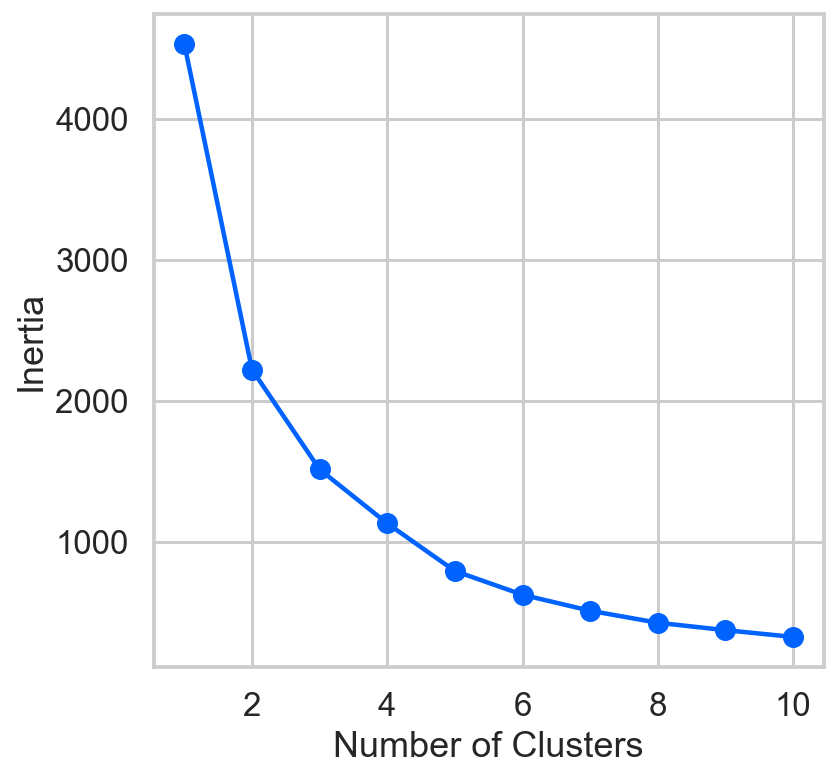
inertia = []
list_num_clusters = list(range(1,11))
for num_clusters in list_num_clusters:
    km = KMeans(n_clusters=num_clusters)
    km.fit(cdf)
    inertia.append(km.inertia_)
    
plt.plot(list_num_clusters,inertia)
plt.scatter(list_num_clusters,inertia)
plt.xlabel('Number of Clusters')
plt.ylabel('Inertia');

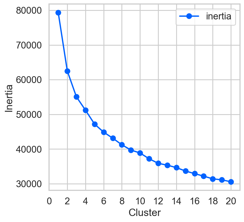
4-2 Comparing in multidimension

km_list = list()
data = StandardScaler().fit(aapl2[float_columns]).transform(aapl2[float_columns])
for clust in range(1,21):
    km = KMeans(n_clusters=clust, random_state=42)
    km = km.fit(data)
    
    km_list.append(pd.Series({'clusters': clust, 
                              'inertia': km.inertia_,
                              'model': km}))

plot_data = (pd.concat(km_list, axis=1).T\
    [['clusters','inertia']].set_index('clusters'))

ax = plot_data.plot(marker='o',ls='-')
ax.set_xticks(range(0,21,2))
ax.set_xlim(0,21)
ax.set(xlabel='Cluster', ylabel='Inertia');

/Users/hun/miniforge3/envs/hun/lib/python3.9/site-packages/pandas/core/indexes/base.py:6982: FutureWarning: In a future version, the Index constructor will not infer numeric dtypes when passed object-dtype sequences (matching Series behavior)
  return Index(sequences[0], name=names)

res = pd.DataFrame()
res['daily_ret'] = aapl2.daily_ret
data = StandardScaler().fit(aapl2[float_columns]).transform(aapl2[float_columns])
km = KMeans(n_clusters=5, n_init=20, random_state=777)
km = km.fit(data)
res['kmeans'] = km.predict(data)

ag = AgglomerativeClustering(n_clusters=5, linkage='ward', compute_full_tree=True)
ag = ag.fit(data)
res['agglom'] = ag.fit_predict(data)

res2 = (res[['daily_ret','agglom','kmeans']]
 .groupby(['daily_ret','agglom','kmeans'])
 .size()
 .to_frame()
 .rename(columns={0:'number'}))
print(res2.to_latex())

\begin{tabular}{lllr}
\toprule
     &   &   &  number \\
daily\_ret & agglom & kmeans &         \\
\midrule
Bear & 0 & 0 &     215 \\
     &   & 1 &      43 \\
     &   & 2 &       1 \\
     &   & 3 &      22 \\
     &   & 4 &       1 \\
     & 1 & 0 &       6 \\
     &   & 2 &       2 \\
     &   & 4 &      18 \\
     & 2 & 0 &       3 \\
     &   & 1 &      88 \\
     &   & 2 &       1 \\
     &   & 3 &     266 \\
     & 3 & 2 &     230 \\
     &   & 4 &       4 \\
     & 4 & 0 &       6 \\
     &   & 1 &     163 \\
Bull & 0 & 0 &     203 \\
     &   & 1 &      40 \\
     &   & 3 &      21 \\
     &   & 4 &       1 \\
     & 1 & 0 &       4 \\
     &   & 2 &       1 \\
     &   & 4 &      13 \\
     & 2 & 0 &      13 \\
     &   & 1 &     114 \\
     &   & 3 &     339 \\
     & 3 & 0 &       2 \\
     &   & 2 &     266 \\
     &   & 4 &       3 \\
     & 4 & 0 &       8 \\
     &   & 1 &     170 \\
\bottomrule
\end{tabular}



/var/folders/1t/_7p_zm4x449blqs7bvqvb0rm0000gn/T/ipykernel_66451/732263353.py:19: FutureWarning: In future versions `DataFrame.to_latex` is expected to utilise the base implementation of `Styler.to_latex` for formatting and rendering. The arguments signature may therefore change. It is recommended instead to use `DataFrame.style.to_latex` which also contains additional functionality.
  print(res2.to_latex())

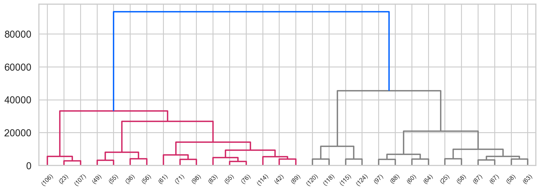
## First, we import the cluster hierarchy module from SciPy (described above) to obtain the linkage and dendrogram functions.
from scipy.cluster import hierarchy
## Some color setup
red,blue = colors[2], colors[0]

Z = hierarchy.linkage(ag.children_, method='ward')
fig, ax = plt.subplots(figsize=(15,5))
hierarchy.set_link_color_palette([red, 'gray'])
den = hierarchy.dendrogram(Z, orientation='top', 
                           p=30, truncate_mode='lastp',
                           show_leaf_counts=True, ax=ax,
                           above_threshold_color=blue)

4-3 utilizing in regression

X_cdf = aapl2[['Close_sp500', 'Close_vix', 'Close_bond_2y']]
data = StandardScaler().fit(X_cdf).transform(X_cdf)
km = KMeans(n_clusters=5, n_init=20, random_state=777)
km = km.fit(data)
aapl['kmeans'] = km.predict(data)[1:]

#### BEGIN SOLUTION
ag = AgglomerativeClustering(n_clusters=5, linkage='ward', compute_full_tree=True)
ag = ag.fit(data)
aapl['agglom'] = ag.fit_predict(data)[1:]

one_hot_encode_cols = ['kmeans','agglom']  ## list of categorical fields
df = pd.get_dummies(aapl, columns=one_hot_encode_cols, drop_first=True).reset_index(drop=True)

## Estimate dtc model and report outcomes
gbc = GradientBoostingClassifier(random_state=777, n_iter_no_change= 10)
gbc = learning(data = df, regressor = gbc, clss = True, pred = True, prnt = False)

gbc2 = GradientBoostingClassifier(random_state=777, n_iter_no_change = 10, n_estimators= gbc.n_estimators_+10)
params = {'max_depth':range(3, len(gbc.feature_importances_), 2),
          'max_features': range(1, gbc.max_features_+1)}
reg = learning(data = df, regressor = gbc2, params = params, clss = True, pred = True)

res = reg.cv_results_
print(reg.best_params_)

Fitting 5 folds for each of 1890 candidates, totalling 9450 fits
Best score: 0.5398230088495575
              precision    recall  f1-score   support

       False       0.51      0.52      0.51       106
        True       0.57      0.56      0.57       121

    accuracy                           0.54       227
   macro avg       0.54      0.54      0.54       227
weighted avg       0.54      0.54      0.54       227

Accuracy: 0.5418502202643172
F1: 0.5666666666666667
AxesSubplot(0.125,0.125;0.62x0.755)
{'max_depth': 17, 'max_features': 17}

4-4 PCA

from sklearn.decomposition import PCA

pca_list = list()
feature_weight_list = list()

## Fit a range of PCA models
data = StandardScaler().fit(aapl2[float_columns]).transform(aapl2[float_columns])

for n in range(6, 10):
    
    ## Create and fit the model
    PCAmod = PCA(n_components=n)
    PCAmod.fit(data)
    
    ## Store the model and variance
    pca_list.append(pd.Series({'n':n, 'model':PCAmod,
                               'var': PCAmod.explained_variance_ratio_.sum()}))
    
    ## Calculate and store feature importances
    abs_feature_values = np.abs(PCAmod.components_).sum(axis=0)
    feature_weight_list.append(pd.DataFrame({'n':n, 
                                             'features': float_columns,
                                             'values':abs_feature_values/abs_feature_values.sum()}))
    
pca_df = pd.concat(pca_list, axis=1).T.set_index('n')
features_df = (pd.concat(feature_weight_list)
               .pivot(index='n', columns='features', values='values'))

features_df

/Users/hun/miniforge3/envs/hun/lib/python3.9/site-packages/pandas/core/indexes/base.py:6982: FutureWarning: In a future version, the Index constructor will not infer numeric dtypes when passed object-dtype sequences (matching Series behavior)
  return Index(sequences[0], name=names)

features	AAPL_factor1	AAPL_factor2	CO	Close	Close_bond_10y	Close_bond_1m	Close_bond_1y	Close_bond_2y	Close_itw	Close_nasdaq	...	ma120	ma20	std120	std20	std_high20	std_intra	std_open20	support_high	support_low	support_open
n
6	0.030236	0.037193	0.008199	0.027970	0.032612	0.032992	0.033682	0.034586	0.026851	0.027899	...	0.032207	0.030129	0.018837	0.018717	0.018823	0.016651	0.019013	0.034963	0.035248	0.037478
7	0.032490	0.032149	0.010461	0.025679	0.029585	0.028476	0.028742	0.029950	0.026914	0.027032	...	0.028294	0.029327	0.019782	0.021357	0.021676	0.026183	0.021668	0.032671	0.031947	0.034375
8	0.036669	0.028255	0.012337	0.022213	0.029923	0.028524	0.029117	0.030328	0.025168	0.023790	...	0.031052	0.026635	0.018100	0.022617	0.022573	0.024953	0.022605	0.030334	0.029549	0.031957
9	0.037665	0.028583	0.028795	0.021349	0.029740	0.027302	0.028086	0.029355	0.023119	0.022945	...	0.033827	0.024899	0.017160	0.021789	0.021669	0.024982	0.021553	0.029501	0.029063	0.031652

4 rows × 35 columns

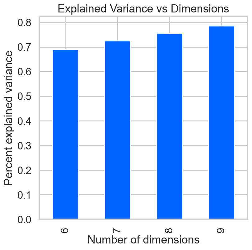
sns.set_context('talk')
ax = pca_df['var'].plot(kind='bar')

ax.set(xlabel='Number of dimensions',
       ylabel='Percent explained variance',
       title='Explained Variance vs Dimensions');

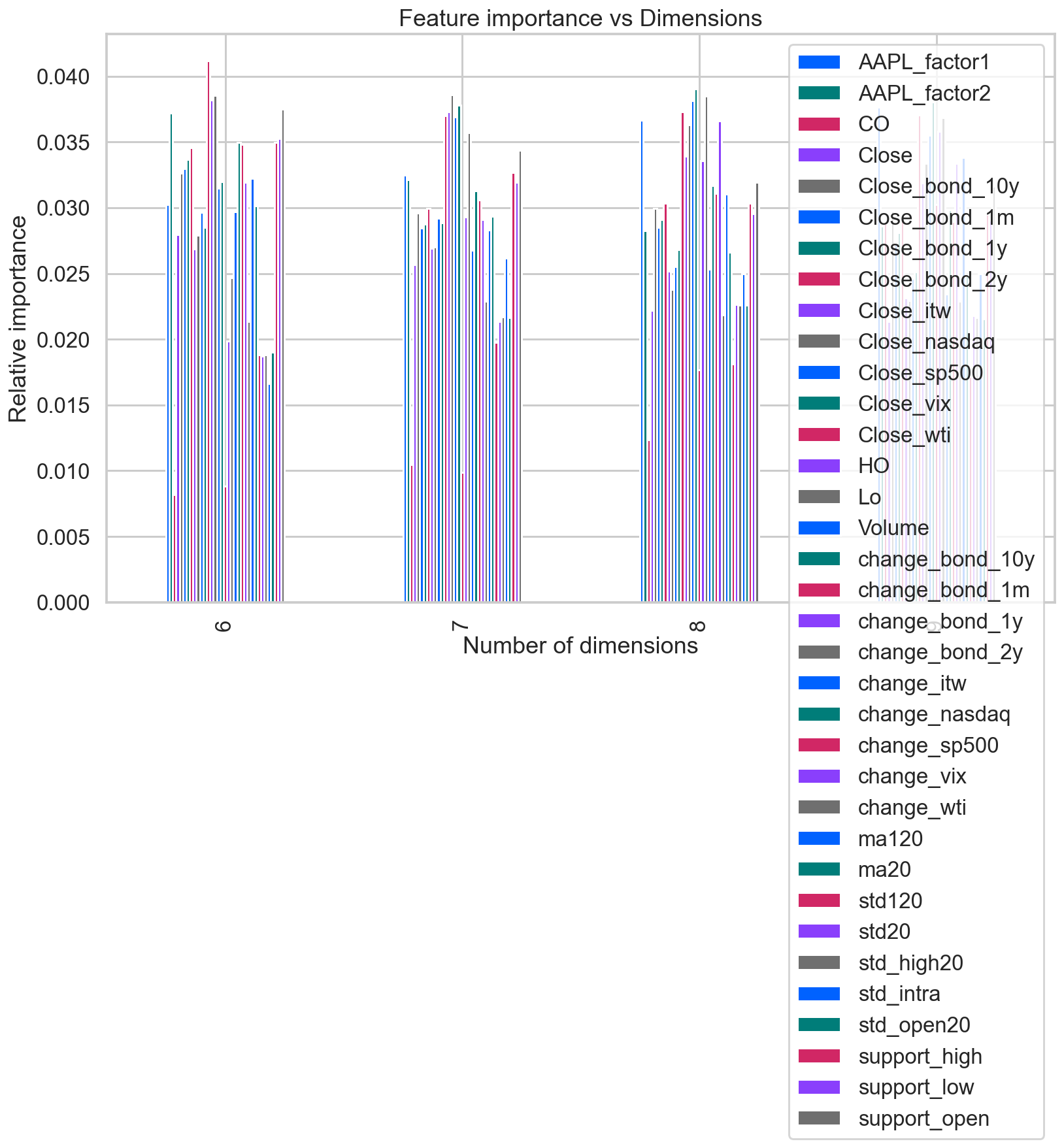
ax = features_df.plot(kind='bar', figsize=(13,8))
ax.legend(loc='upper right')
ax.set(xlabel='Number of dimensions',
       ylabel='Relative importance',
       title='Feature importance vs Dimensions');

from sklearn.decomposition import KernelPCA
from sklearn.model_selection import GridSearchCV
from sklearn.metrics import mean_squared_error

## Custom scorer--use negative rmse of inverse transform
def scorer(pcamodel, X, y=None):

    try:
        X_val = X.values
    except:
        X_val = X
        
    ## Calculate and inverse transform the data
    data_inv = pcamodel.fit(X_val).transform(X_val)
    data_inv = pcamodel.inverse_transform(data_inv)
    
    ## The error calculation
    mse = mean_squared_error(data_inv.ravel(), X_val.ravel())
    
    ## Larger values are better for scorers, so take negative value
    return -1.0 * mse

## The grid search parameters
param_grid = {'gamma':[0.001, 0.01, 0.05, 0.1, 0.5, 1.0],
              'n_components': [2, 3, 4]}

## The grid search
kernelPCA = GridSearchCV(KernelPCA(kernel='rbf', fit_inverse_transform=True),
                         param_grid=param_grid,
                         scoring=scorer,
                         n_jobs=-1)


kernelPCA = kernelPCA.fit(data)

kernelPCA.best_estimator_

KernelPCA(fit_inverse_transform=True, gamma=0.05, kernel='rbf', n_components=4)

kernelPCA.best_estimator_.eigenvalues_

array([163.71226988, 144.0926473 ,  93.50586323,  65.88489674])

from sklearn.pipeline import Pipeline
from sklearn.preprocessing import StandardScaler
from sklearn.linear_model import LogisticRegression
from sklearn.metrics import accuracy_score


X = aapl2[float_columns]
y = aapl2.daily_ret
sss = TimeSeriesSplit(n_splits=5)

def get_avg_score(n):
    pipe = [
        ('scaler', StandardScaler()),
        ('pca', PCA(n_components=n)),
        ('estimator', LogisticRegression(solver='liblinear'))
    ]
    pipe = Pipeline(pipe)
    scores = []
    for train_index, test_index in sss.split(X, y):
        global X_train, y_train
        X_train, X_test = X.iloc[train_index], X.iloc[test_index]
        y_train, y_test = y.iloc[train_index], y.iloc[test_index]
        pipe.fit(X_train, y_train)
        scores.append(accuracy_score(y_test, pipe.predict(X_test)))
    return np.mean(scores)


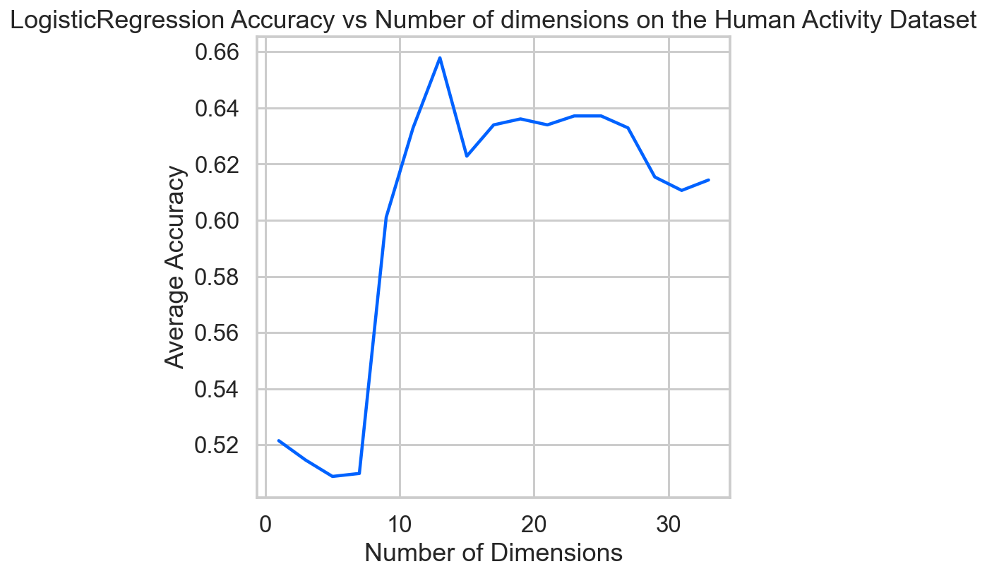
ns = np.arange(1, 35, 2)
score_list = [get_avg_score(n) for n in ns]

sns.set_context('talk')

ax = plt.axes()
ax.plot(ns, score_list)
ax.set(xlabel='Number of Dimensions',
       ylabel='Average Accuracy',
       title='LogisticRegression Accuracy vs Number of dimensions on the Human Activity Dataset')
ax.grid(True)

ETC

### How to make pipeline by features?

from sklearn.pipeline import make_union, make_pipeline
from sklearn.preprocessing import FunctionTransformer

def get_text_cols(df):
    return df[['name', 'fruit']]

def get_num_cols(df):
    return df[['height','age']]

vec = make_union(*[
    make_pipeline(FunctionTransformer(get_text_cols, validate=False), LabelEncoder()))),
    make_pipeline(FunctionTransformer(get_num_cols, validate=False), MinMaxScaler())))
])