Clustering Algorithms

Distant Metrics

Manhattan Distance, L1 distance

Another distance metric is the L1 distance or the Manhattan distance, and instead of squaring each term we are adding up the absolute value of each term. It will always be larger than the L2 distance, unless they lie on the same axis. We use this in business cases where there is very high dimensionality.

As high dimensionality often leads to difficulty in distinguishing distances between one point and the other, the L1 score does better than the L2 score in distinguishing these different distances once we move into a higher dimensional space.

Euclidean Distance, L2 distnace

$${\displaystyle d(p,q)={\sqrt {(p_{1}-q_{1})^{2}+(p_{2}-q_{2})^{2}+\cdots +(p_{i}-q_{i})^{2}+\cdots +(p_{n}-q_{n})^{2}}}.}$$

L2 norm

$${\displaystyle \|{\boldsymbol {x}}\|_{2}:={\sqrt {x_{1}^{2}+\cdots +x_{n}^{2}}}.}$$

Cosine Distance

Cosine is better for data such as text where location of occurence is less importance. Also, it is more robust than euclidean distance, which is vulnerable in multi-dimension. Cosine is better for data such as text where location of occurrence is less important.

$$cos(\theta)=\frac{\vec{x} \cdot \vec{y}}{\|\vec{x}\| \|\vec{y}\|}$$

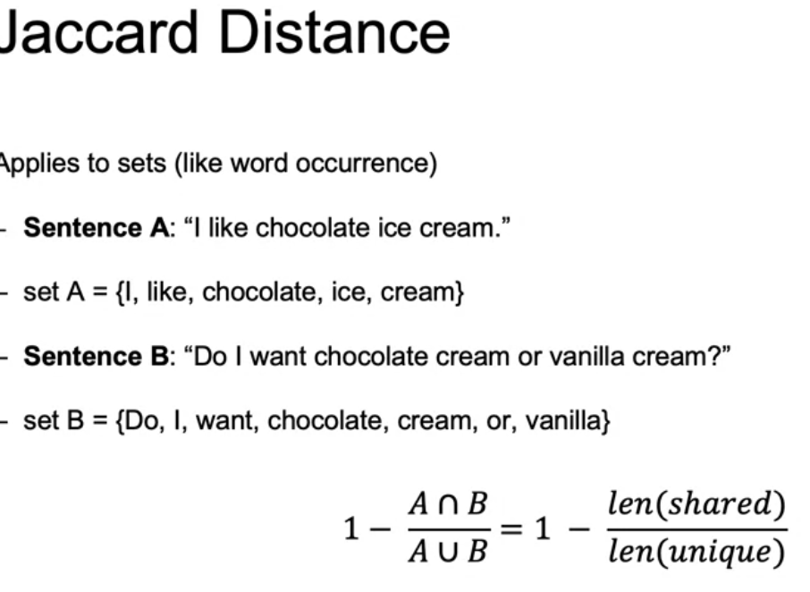
Jaccards Distance

Clustering Algorithms

Hierarchical Agglomerative Clustering

1. Find closet pair and merge them.
2. We get clusters and regard it as a point. For distance between clusters, use average distance regarding all the point within their respective clusters.
3. Repeat 1 and 2 until we get a single cluster.

Average cluster distance

For the new combined cluster, cluster distance will be increased. Some cluster will merged with larger value of cluster distance. When all the distance is above a threshold, we stop clustering.

Single linkage

Minimum pairwise distance between clusters Pro is a clear separation of clusters. Con is that seperation is vague with outliers failing close to certain clusters.

Complete linkage

We take maximum value. Pro better seperating even with noise. Cons tend to break apart big clusters.

Average linkage

Both Pro and Cons of Single and Complete

Ward linkage

merge based on best inertia.

Code

from skleran.cluster import AgglomerativeClustering
agg = AgglomerativeClustering(n_clusters=2, 
                              affinity='euclidean', 
                              linkage='average')
agg.fit(X)
y_predict = agg.predict(test)

DBscan

Density Based Spatial Clustering of Applications with Noise Points are clustered using density of local neighborhood so that it finds core points in high density regions adn expands clusters from them. Algorithm ends when all points are either classified into cluster or noise

1. Randomly select from high density reagions.
2. Find Core, Density reachable points.
3. Repeat 1,2 until all points are clustered, find Noise(Outlier).

• Required inputs: Metric, Epsilon of neighborhood, N_clu (determines density threshold for fixed $\epsilon$)
• Outputs:
  • Core: points that has more than n_clu neighbors in ther $\epsilon$ neighborhood
  • Density reachable: $\epsilon$ neighborhood of core points that has fewer than n_clu neighbors itself
  • Noise: no core points in its $\epsilon$ neighborhood

Char

Pro
No need to specify number of clusters. Allows for noise. Can handle arbitrary shaped clusters
Con
Requires two parameters, Finding appropriate epsilon and n_clu.\

Code

from skleran.cluster import DBSCAN
db = DBSCAN(eps=3, min_samples=2)
db.fit(X)
clusters = db.labels_ #outlier labed as -1

Mean Shift

Mean Shift is similar to KMeans, but centroid is the point of highest local density. Algorthm finish when all points are assigned to a cluster.

1. chose point and window W
2. calculated weighted mean in W
3. Shift centroid of window to new mean
4. repeat 2~3 until convergence, until the point with local density maximum(mode) is reached
5. repeat 1~4 for all data points.
6. Data points that lead to same mode are grouped into same cluster.

Weighted mean

Commonly, kernel function that used is RBF kernel.

$$m(x) = \frac{\sum_{x_i \in W} x_i K(x_i-x)}{\sum_{x_i \in W} K(x_i-x)}$$

char

Pro
model free, one parameter(window size), robust to outliers Con
depend on window(bandwith), slection of window is hard to find.

Code

from skleran.cluster import MeanShift
ms = MeanShift(bandwidth=2)
ms.fit(X)
ms.predict(Test)

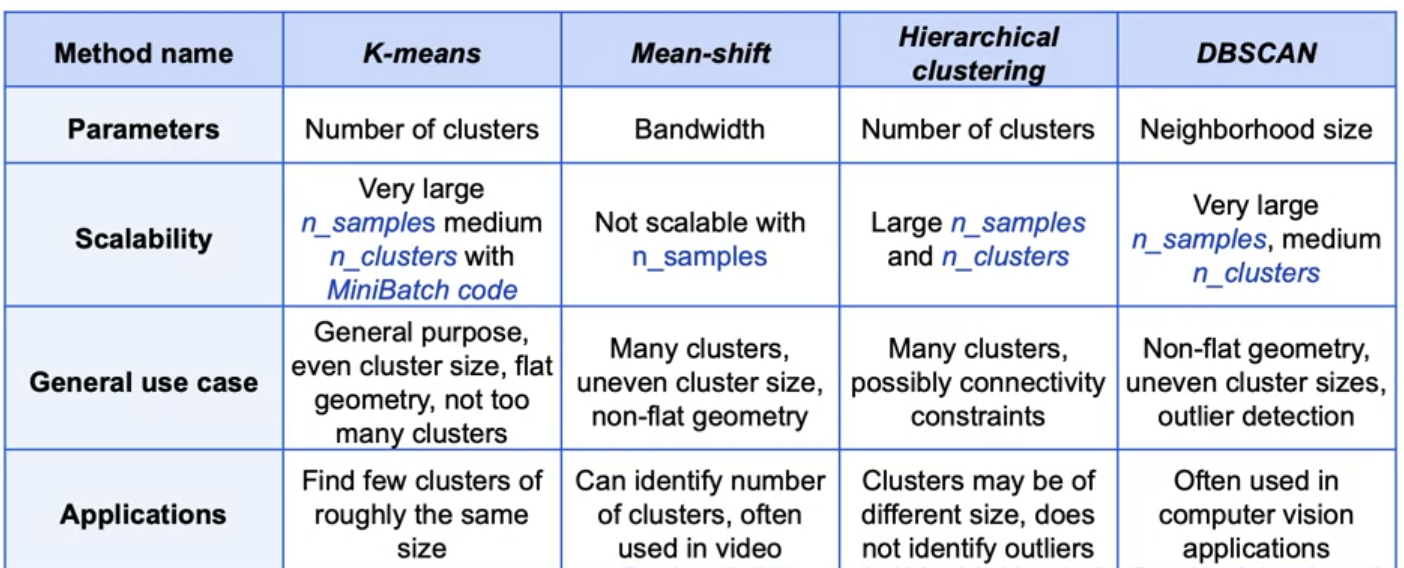
Summary