Dimensionality Reduction

Dimensionality ReductionPermalink

Too many features leads to worse performance. Distance measures perform poorly and the indicent of outliers increases. Data can be represented in a lower dimensional space. Reduce dimensionality by selecting subset (feature elimination). Combine with linear and non-linear transformation.

PCAPermalink

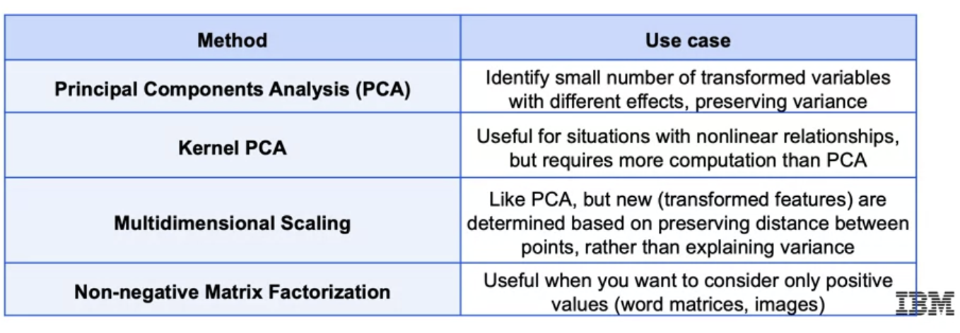
Principal Component Analysis (PCA) is a dimensionality reduction technique. It is a linear transformation that projects the data into a lower dimensional space. Let direction $v_1$ and length $\lambda_1$ be the first principal component. $v_1$ is perpendicular to $v_2$ which has length $\lambda_2$.

SVDPermalink

Principal components are calculated from $V$
Truncated SVD is used for dimensionality reduction from n to k
Variance is sensitive to scaling .

from sklearn.decompositon import PCA
PCAinst = PCA(n_components=2) #create instance
x_trans = PCAinst.fit_transform(x_train) #fit the instance on the data

Non-linearPermalink

Kernel PCAPermalink

Use kernel trick introduced in SVM to map down linear relationship.

from sklearn.decomposition import KernelPCA
kPCA = KernelPCA(n_components=2, kernel='rbf', gamma=0.04)
x_kpca = KPCA.fit_transform(x_train)

Multi-Dimensional Scaling (MDS) Permalink

MDS maintains the distance between points in a low-dimensional space.

from sklearn.decomposition import MDS
mds = MDS(n_components=2)
x_mds = mds.fit_transform(x_train)

Others: Isomap, TSNEPermalink

Non-negative Matrix Factorization Permalink

Decompositing matrix only non-negative values. For example, vectorized words, images. Let $V = W\tiems H$ so that $term-documentMatrix = Term\to Topics + Topic\to Docs$. Also in Image, we can compress only shaded values.
Can never undo the application of a latent feature, it is much more careful about what it adds at each step. In some applications, this can make for more human interpretable latent features.
Thus NMF are non othogonal.

from sklearn.decomposition import NMF
nmf = NMF(n_components=2, init='random')
x_nmf = nmf.fit(x)

SummaryPermalink

Example of Dim RedcutionPermalink